Use GridSearchCV to Tune ML Models

Series: Taiwan Credit Default Risk Dataset

Series: Taiwan Credit Default Risk Dataset

This article is part of a series where we explore, preprocess, and run several machine learning methods on the Taiwan Credit Default dataset. The dataset can be found here: dataset .

In a previous article, we used XGBoost as a way to identify the most important features in the dataset, in terms of

the KFold algorithm to help discover the relative merits of several machine learning algorithms for a binary classification task. Specifically, the task is to predict whether a given credit customer will default on their payments or not. KFold allowed us to quickly run several bare-bones models on the data and plot the results to help narrow down one or two promising candidates for further development.

First, let’s import some of the packages we will need.

Next, we will import the dataset we prepared in the last article. It has one-hot encoding applied to the categorical features and standardized scaling applied to the numeric features. The code below will read the CSV file into a Pandas dataframe. We set the index_col parameter to 'ID' to retain the index from the original file.

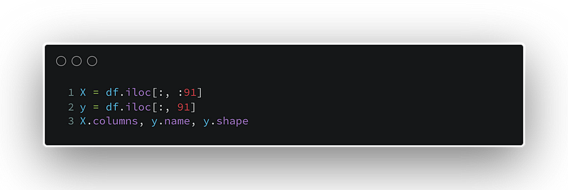
The dataframe must be separated so that the features are together and the labels, or targets are alone. Below, we use Pandas to achieve this.

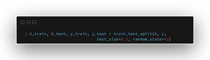
Now, we will split our data into training and test datasets. Each pair has the X, for the features, and y for the labels. The random_state is set to ensure reproducibility of our results if others want to simulate our steps.

The next step we are going to take is to produce a baseline model for this binary classification task. To do this, we choose the Logistic Regression algorithm, which performed near the top of our results last time. The parameters are what we saw as most successful in the last article.

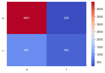
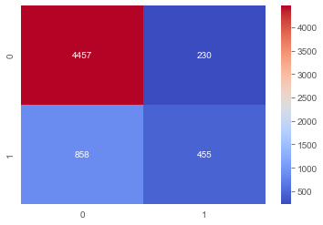
We look at the confusion matrix for the Logistic Regression classifier and see that the majority class, 0, has the most accurate predictions by far. As it turns out, there are many more 0’s in the dataset than 1’s. This kind of class imbalance can lead to problems with modeling. In a future article, we will look at some potential solutions for class imbalance.

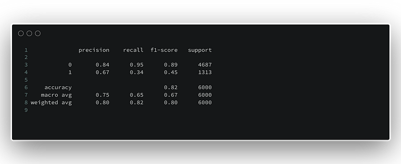
The classification_report gives details about the precision, recall, and f1-score for the model. We can see the accuracy is about 82%.

Hyperparameters can be notoriously difficult, and time-consuming, to tune. With GridSearchCV we can compare the performance of several versions of the same base classifier on the same task. We instantiate a classifier object, then hand the parameter grid to it.

Each line of the param_grid has a set of hyperparameter settings that defines the base model further. GridSearchCV runs each model on the dataset, and produces a set of attributes. We can access the attributes, like best_params, to show which configuration works best.

Below, we experiment with different regularization settings and tolerances on the Logistic Regression model. Also, the upcoming XGBoost Classifier parameter grid is defined.

Here, we define the GridsearchCV instance for the Logistic Regression classifier and run the fit method with the training data.

Instead of evaluating the models on the basis of simple accuracy, we have decided to use the roc_auc score. Looks like the best configuration for Logistic Regression is the following:

Now, we discover the best configuration for XGBoost below:

We know better now the best version of each model for this dataset, given the parameters we decided to evaluate. In order to evaluate a classifier’s performance in this case, we could settle for the simple accuracy score. However, we have already observed a significant imbalance between the two classes in the dataset. In cases like this, roc_auc will allow us to assess performance in a more robust way.

The ROC-AUC Curve plot below compares the Logistic Regression classifier to the XGBoost Classifier in terms of the the area under the curve of the ROC, or Receiver Operator Characteristic. For imbalanced datasets in binary classification tasks, this is generally a better measure of a model’s performance than standard accuracy.

The red dashed line represents the XGBoost classifier and the orange line shows the Logistic Regression classifier. The diagonal blue line is the 50% mark, below which the model performs worse than a random guess.

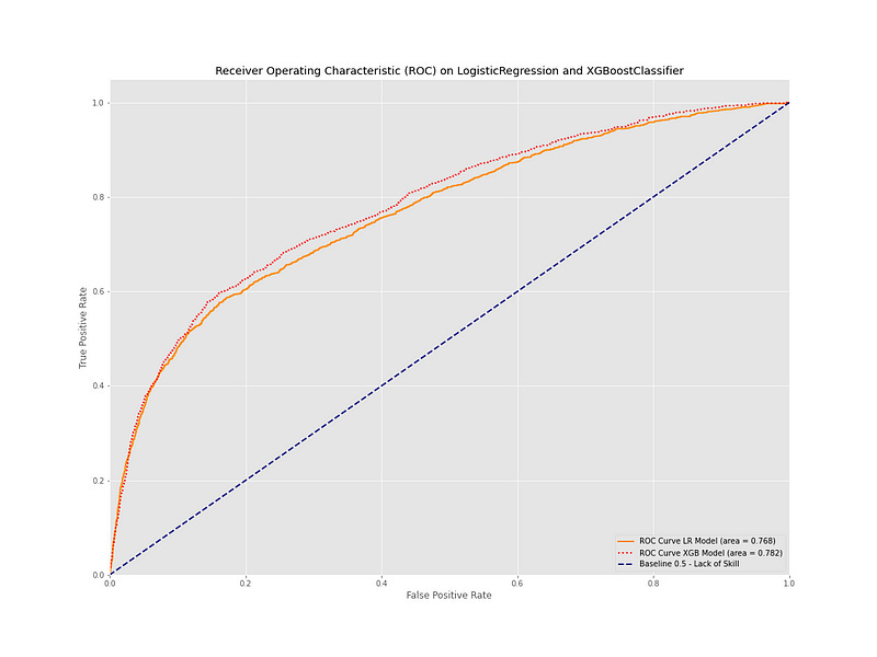
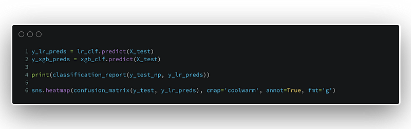
We can see that the XGBoost classifier has the edge, as it covers a bit more area of the whole. To see a detailed, numeric representation, we can generate the actual label predictions for each classifier with their respective predict methods. Scikit-learn has the classification_report which displays a breakdown of of precision, recall, f1-score, and accuracy.

precision    recall  f1-score   support

           0       0.84      0.95      0.89      4687
           1       0.66      0.35      0.46      1313

    accuracy                           0.82      6000
   macro avg       0.75      0.65      0.67      6000
weighted avg       0.80      0.82      0.80      6000

For a visually appealing display of the ability of the classifier to predict each class, the confusion_matrix is useful. We make the graph from the data provided by the Scikit-learn confusion_matrix module. Then, we use seaborn and its heatmap graph to make the point visually, with the actual numbers for each class presented. This makes it easy to see the general point and also be able to analyze more in terms of specific data.

precision    recall  f1-score   support

           0       0.84      0.95      0.89      4687
           1       0.68      0.35      0.47      1313

    accuracy                           0.82      6000
   macro avg       0.76      0.65      0.68      6000
weighted avg       0.81      0.82      0.80      6000

Evaluated from these standpoints, the two classifiers are almost identical. Both have similar scores for each class and accuracy is identical. However, the XGBoost classifier shows slightly more promise. First, it has more correct predictions of both the 0 and 1 classes. Also, the false positive and false negative rates are lower. In the case of assessing default risk, it is better to keep the false positive rate as low as possible.

These gains in accuracy and performance are admittedly modest. Earlier, we noted the sizable imbalance in the classes. There are several strategies for dealing with class imbalance and it seems worthwhile to explore some options to improve our predictive power.

In the next article, we will look into using two techniques called SMOTE and Neighborhood Cleaning Rule to apply some sampling methods to address the imbalances in the dataset and hopefully improve performance.