
Preparing Data for ML & Deep Learning
Series: Taiwan Credit Default Dataset

Series: Taiwan Credit Default Dataset
This article is part of a series where we explore, preprocess, and run several machine learning methods on the Taiwan Credit Default dataset. The dataset can be found here: dataset .
For any dataset we work with, it must be cleaned up and transformed so we can use it for building models and/or deriving insights from visualizations. This step, often called “data preprocessing”, or “data wrangling”, goes together with the overall process of EDA, or exploratory data analysis. Ultimately, to gain optimal value from our data, we need to know what is in the dataset: details about the features, such as data type, and encoding; and as much as possible about the potential of the data to teach us.
The example we will use in this article is a dataset from 2005 (link is above) which shows details on credit card default in Taiwan over the span of a few months. Twenty-three features were collected, with a mixture of categorical and numeric variables. A single binary column gives the target variable, for which 0 stands for ‘no default’ and 1 for ‘default. I suggest reading the brief on the dataset at the link above to gain more knowledge of the dataset, which is from the well-known UCI Machine Learning data repository.
Let’s get started by importing the dataset into Pandas:
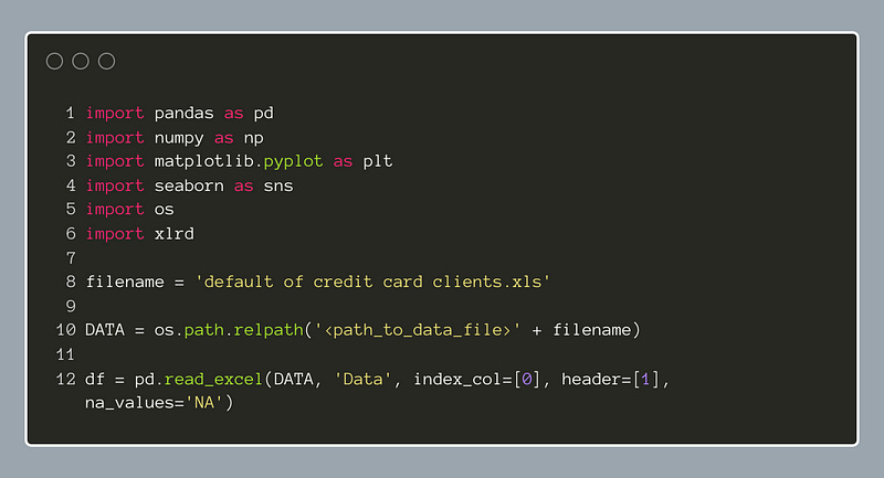
Notice here we have imported the xlrd package. This package helps importing an older Microsoft Excel file type, the xls file. It may have to be installed in your Python environment; in which case we should be able to install it with pip.
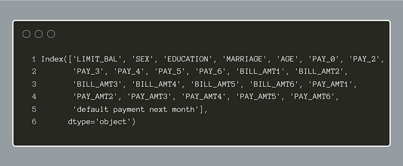
The dataframe column names are below:
We know from the dataset description that the last column, ‘default payment next month’, is our target variable. Before we transform the data, it may be simpler to separate the ‘X’ data, that is the features, from the ‘Y’, target data. Below, we use the Pandas indexer, iloc, to make two dataframes, ‘X’ and ‘Y’:

We will operate on ‘X’ and leave ‘Y’ aside for now.
Next, we will prepare the data for general machine learning and deep learning model building. When we read the dataset description, we gathered which features are categorical, and which are numeric.
The categorical features in this dataset use integers to encode the categories. Even though these are technically numbers, if we want the categorical nature of each to be represented, it will help to encode them. There are several different methods for encoding categorical features. In this instance, I have chosen one-hot encoding. This method will take a single categorical feature and create a new set of features where each represents the presence or absence of a given category.
For example, the ‘MARRIAGE’ feature in this set has three possible values: (1, 2, 3). The OneHotEncoder from SciKit-Learn will create three new features that can only have two values, 0 or 1. These indicate absence or presence of that specific category within the instance, or row, of the dataset. The overall result is a sparser representation of the same information. Later, this will likely help any machine learning models or neural networks we use to understand the data better.
To handle the numeric features, we will apply the StandardScaler to them. This is designed to standardize the features so that the overall dataset has a relatively similar range. It will find the mean and standard deviation of each feature, subtract the mean, and then divide by the standard deviation. This operation is simple and common when preparing data; it retains the variance of the features but places it within a common scale.
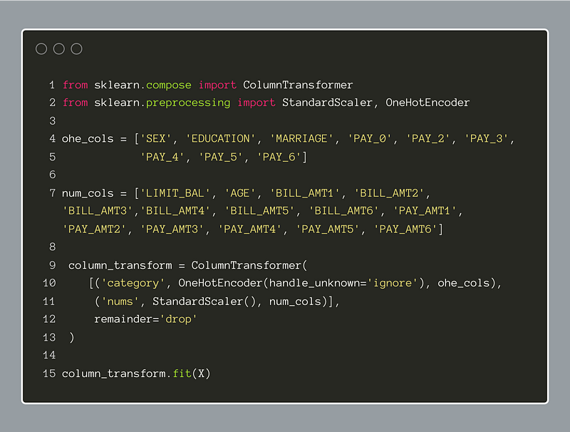
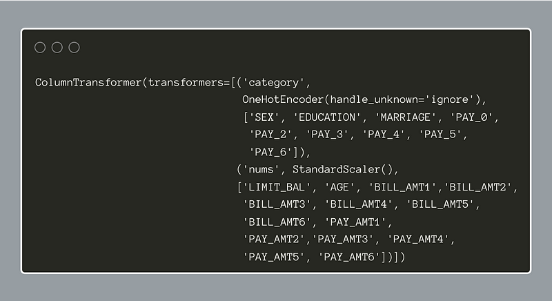
In the code below, we have created two lists, one for the categorical features and one for the numeric (continuous) feature names. Doing this beforehand will make running the transformations easier. Now, we can use the SciKit-Learn ColumnTransformer to construct a dual-pronged transformer to apply the chosen transformations to each subset of columns. The use of the “remainder=’drop’” parameter within the ColumnTransformer will exclude the original features from the resulting dataframe. It should be noted as well that the string placed in the first position of each transformer definition will be the prefix for each of the new features created.
After defining the ColumnTransformer, we run the fit method on the ‘X’ dataframe:
Below, the configuration of the ColumnTransformer object is shown:
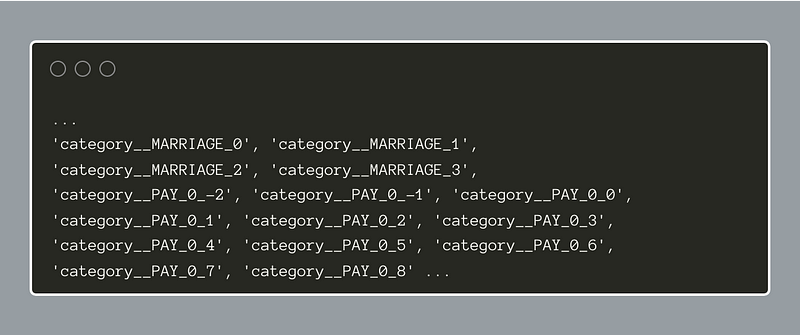
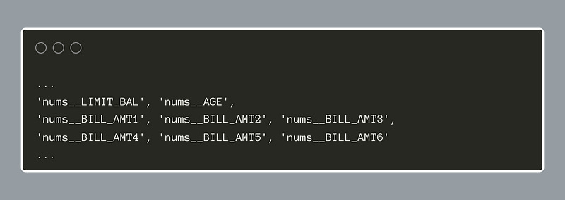
A call to the get_feature_names_out method will display all the new feature names. A truncated list is shown below for brevity’s sake.

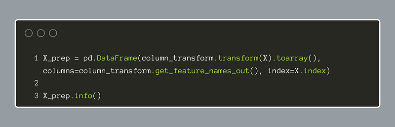
Now, we need to create a new transformed dataframe. We use Pandas to create a new ‘X_prep’ dataframe. Notice we can simply call the transform(X).toarray() method to give the new dataset and the .get_feature_names_out() method to feed in the new column names. The prior index is retained by specifying the index=X.index . Calling info() on the new dataframe reveals all of the columns and their data types. When we do this, we will see that every column is a floating-point number.
The next to last step is to concatenate the new X_prep features to the target column, Y. The code below will achieve this, and we will have a dataframe of features combined with the target variable.

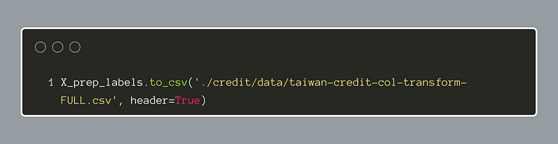
For easy use with most of the upcoming work at creating machine learning models and so forth, it makes sense to write the new standardized and one-hot encoded dataset into a CSV file. Then, we will have the same dataset to start with for each of our models with no need to repeat the initial processing.
In the next episode, we will load this dataset from the file and continue to get acquainted with the data and see how some basic machine learning models perform on it.