

XGBoost & KFold for ML Model Selection
XGBoost & KFold for ML Model Selection
How to use XGBoost to select top features, then KFold to select a model.

Series: Taiwan Credit Default Dataset
This article is part of a series where we explore, preprocess, and run several machine learning methods on the Taiwan Credit Default dataset. The dataset can be found here: dataset .
Two important questions usually come up when we are trying to figure out how best to model a dataset, and hopefully make predictions based on it:
· Are all the given features relevant, and if not, which subset will be best?
· Given the best subset of features, which machine learning model will yield the best results?
Because of the limitations of computing power, even now in 2022, it is important to reduce the number of dimensions to as few as possible, without sacrificing significant amounts of information. In this article we will look at one strategy for selecting the best subset of features, using the XGBoost algorithm. Then, we will use the resulting subset of data to evaluate several basic classifiers to decide which deserves more time tuning for optimal performance. Let’s get started!
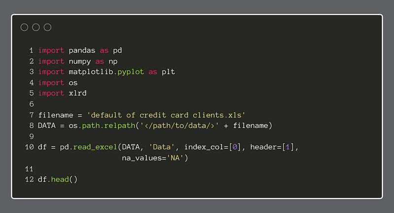
The first step is to import some initial packages and import the data from Excel. Below, we have imported the data into Pandas with a helper application, xlrd. This will allow us to import .xls files, and even select the specific sheet in the workbook. This produces a dataframe with 24 columns with 30,000 instances. For a more detailed look at this dataset, see this article .
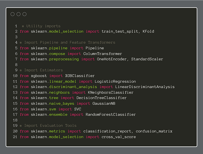
Now, we will import most of the packages, most from Scikit Learn, that we will use going forward.
This short piece of code will separate the features from the target variables.

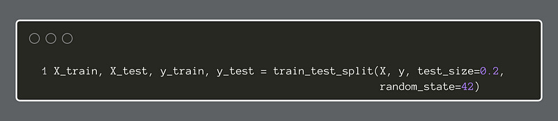
Our next step is to use train-test-split to give us subsets of the data to train and test our models. We will use an 80/20 split (20% is testing data) and set a random_state of 42, which seems to be somewhat of a tradition.
There are several ways to identify the best subset of features to select for training a model. The basic concept is that we want to retain those features with the most importance for predicting the target variable and leave off the rest of the features that do not benefit the prediction task enough to warrant the added complexity. Complexity can entail overfitting, difficulty of interpretation, and excessive resource needs. Therefore, we will want to minimize it.
For this example, we will use the popular XGBoost algorithm in classifier mode. Here, we fit the model to the training data and then use the feature_importances_ attribute to discover the features that retain the most explanatory variance, while minimizing the number of features. At a certain point, some features yield less explanatory power than they are worth in terms of complexity.
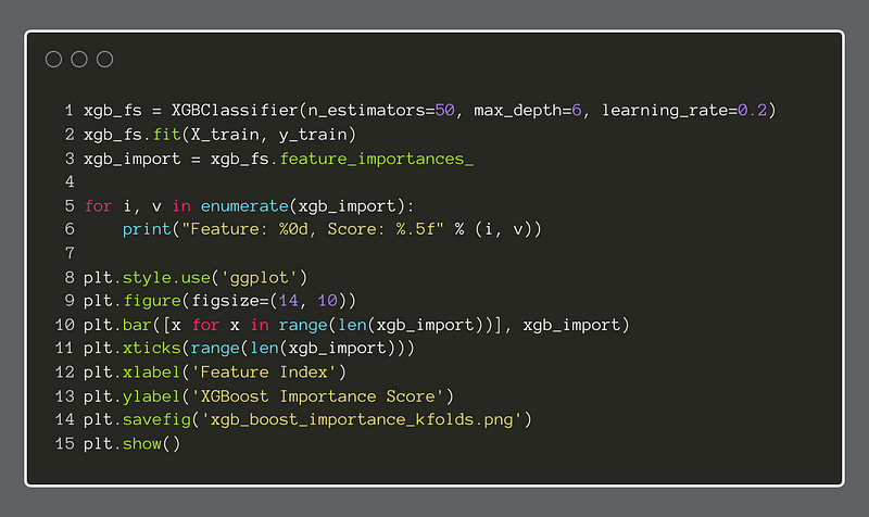
The plot below shows the index numbers of each feature in the dataframe and what relative importance each has in predicting the target variable.
According to this analysis, two features appear to hold a larger share of the predictive weight. Now, it should be noted that by adjusting the n_estimators, learning_rate and/or the max_depth in the XGBClassifier, we may see some features become slightly more prominent. Altogether, for this example, this configuration worked well.
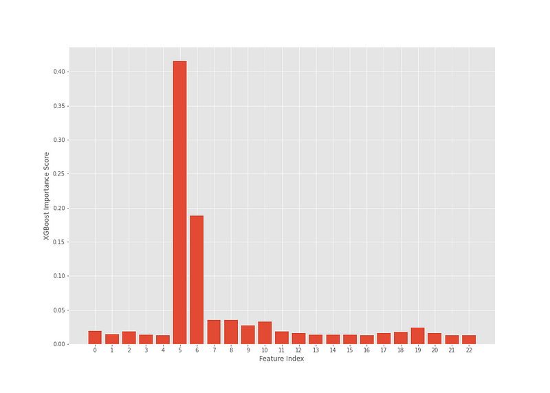
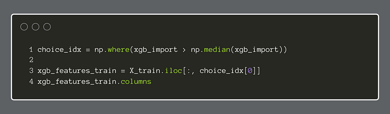
Instead of just picking the top features by sight, we can use a formula of some kind to pick them for us. In this example, we chose to select all features that were greater than the median of all feature importances.
Now, we will fetch the feature names, to make it easier to refer to them in the next steps.

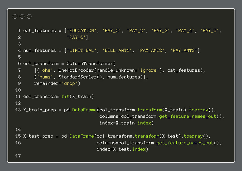
Of those features we decided to retain, some are categorical while others are continuous numeric features. Therefore, we will want to apply a different type of transformation to each so that the models can use the data well. To do this, we will use the Scikit Learn ColumnTransformer to apply the transformations appropriately.
There are several ways to prepare categorical data for modeling. In this case, we will apply the OneHotEncoder to all categorical features. Since we decided to be selective about the features we retained, the complexity burden will thereby be lessened. For each categorical feature, the OneHotEncoder will create a new feature for every binary outcome within the original feature. For instance, if a column has 4 possible categories, the OHE creates 4 columns and then puts either 0 or 1 in each row to declare whether that category is absent or present in that row. We end up with a sparse data representation that accounts for the categories but is more easily used by models.
For the numeric features, we will keep it simple and apply the StandardScaler to them. This standardizes each feature to remove the mean and scale to unit variance. With this transformation, the data will not be as susceptible to outliers. There are other types of scaling, such as the MinMaxScaler, but we will use the StandardScaler.
We apply the column transformations to both the training and test data for X with the fit method.
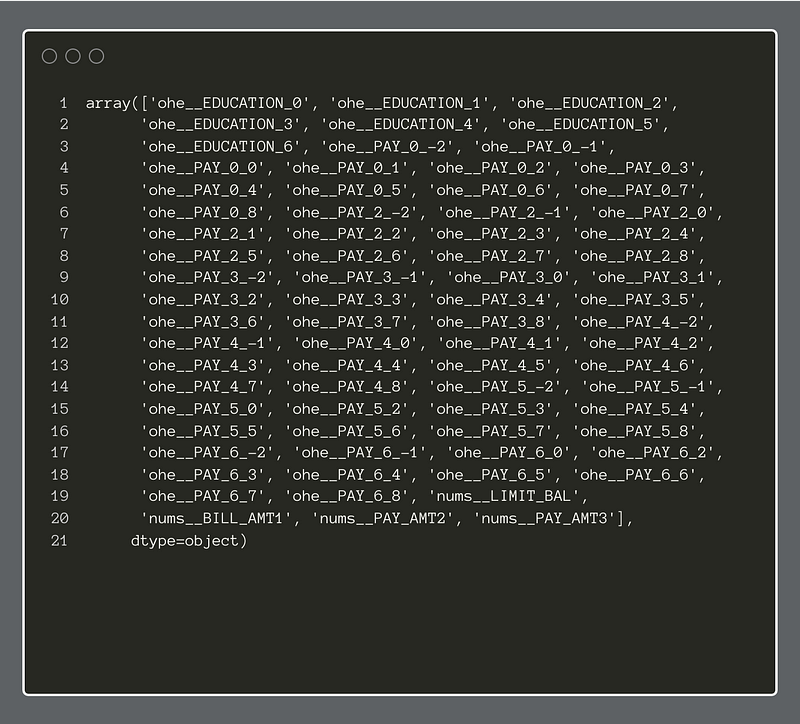
We can see the new feature names of the transformed dataset below:
With the data pared down to more essential features and transformed for use in machine learning models, we move on to create the apparatus to test a series of classifiers side-by-side, to get a better idea as to which one(s) will be worth investigating further. This step is often called model selection. The models, for the most part, do not have any hyperparameter changes. We run a vanilla version of each to attempt to get a ballpark estimate of the relative merits of each.
The steps below were borrowed from, and inspired by, the book, Machine Learning and Data Science Blueprints for Finance by Hariom Tatsat, Sahil Puri, and Brad Lookabaugh (O’Reilly, 2021), 978–1–492–07305–5.
I recommend reading it. It has succinct and useful descriptions of common techniques in ML, especially for the financial domain.
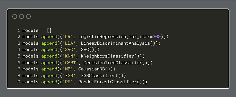
The first step is to create a Python list, and then append each of our candidate classifiers to it.
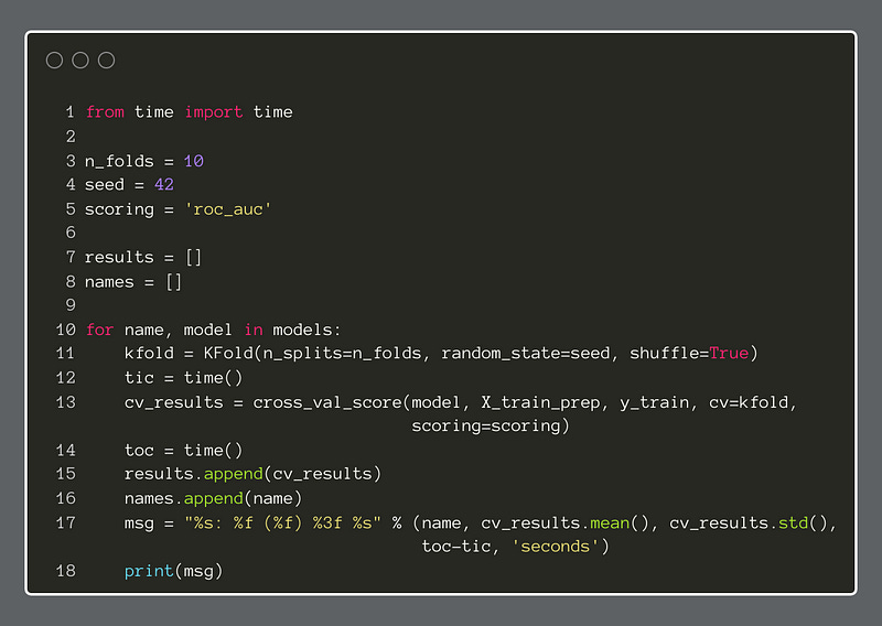
Next, we set parameter values, like n_folds and scoring for the KFold cross-validator. Here, the choice of roc_auc as a scoring metric is important. Our task is supervised binary classification, which means we have access to the target variable, and it is a binary choice, 0 or 1.
The Area Under the Curve of the Receiver Operating Characteristic graph is well-suited to this classification task. It plots the true positive rate against the false positive rate while varying a discrimination threshold. The score is the area of the graph that is under the line produced. The perfect score is 1.0 and a not-so-good score is anywhere below 0.5. The lower the score, the worse the classifier performs. Also, a score below 0.5 indicates that the classifier shows no real ability to predict the target.
Finally, we will import the Python time module to be able to compute the seconds that elapse for running each classifier. We print the results to the console.
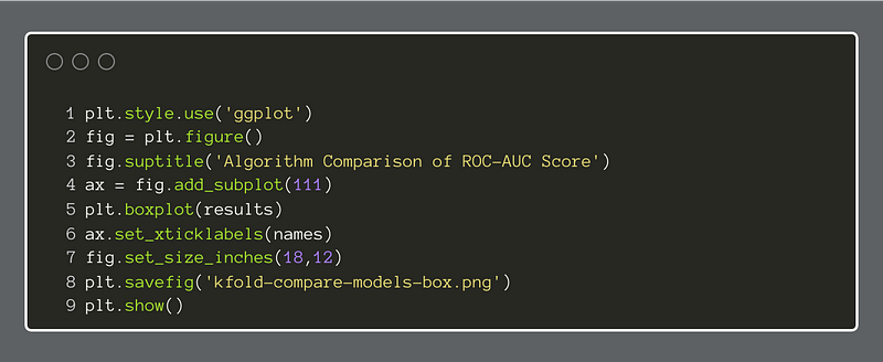
Finally, we will make a series of boxplots to help us compare the different classifiers.
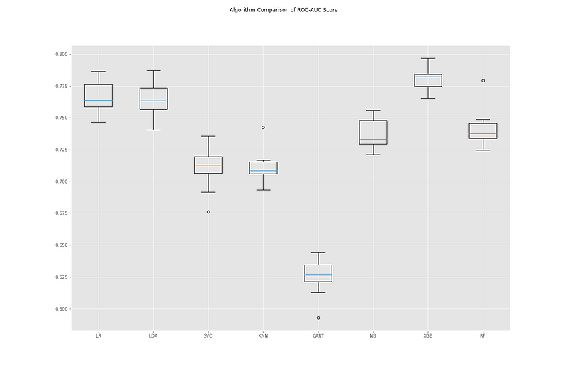
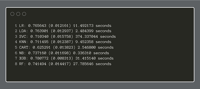
Compared side-by-side, we can see that the XGBoost classifier performed better than the others. Sharing second place, Logistic Regression and Linear Discriminant Analysis show promise. With this information, we can go on to focus on one or two of these classifiers and tune their respective hyperparameters. By using this method upfront, we save time and energy by focusing on developing models that show genuine potential for performing the task at hand.
In another article, we will do just that and see how well one of these non-neural network approaches can classify credit default instances.